link to the repo
Modul gbsv FHNW
Part 1: Correlation in Signals
Overarching Task: Choose a country and theme all the MC tasks to this county. The use cases, problem statements, signals and images should be related to your country of choice. It can be the same country as in MC1, but you may also choose a different one.
1: Exploring the Audio Landscape
Day 1 Task:Suitable for your country: Define a use case to recognize whether a 1D signal contains recurring patterns. Find a suitable 1D signal (audio, time series, vital signs, ...) that contains recurring patterns to apply auto-correlation in the following days.
Implementation:
first all needed imports are made and the signal is loaded and inspected
import time
import cv2
import librosa
import matplotlib.pyplot as plt
import numpy as np
import pandas as pd
import sounddevice as sd
from scipy.io.wavfile import write
from scipy.signal import correlate, find_peaks
from scipy.fftpack import fft
from IPython.display import Markdown, Audio
from rich import print
audio, sample_rate = librosa.load("sound/bell.wav")
print(f"this is what the audio looks like. {audio}")
print(f"The dimension: {audio.shape}")
print(f"audio min: {np.max(audio)} and audio max: {np.min(audio)}")
display(Markdown(f"**ring the Bell**"), metadata={"tags": "audio"})
display(Audio(audio, rate=sample_rate))
this is what the audio looks like. [2.6749703e-35 8.3550063e-35 1.1725352e-34 ... 6.8832678e-04 7.8442483e-04 0.0000000e+00]
The dimension: (1641260,)
audio min: 0.8644417524337769 and audio max: -0.8645315766334534
ring the Bell
The chosen use case is to estimate the weight/size of a Swiss cowbell based on its frequency characteristics using auto-correlation. Cowbells produce distinct resonant frequencies determined by their size, material, and weight. Identifying recurring patterns in their acoustic signal can help derive these physical properties. i chose this sound because cowbells are an iconic symbol of Swiss craftsmanship and tradition, and we can always hear them on our hiking trips on weekends. The objective of this experiment is to demonstrate whether auto-correlation can reliably detect these recurring patterns and link them to the bell’s weight. The chosen signal is a recording of a Swiss cowbell.
2: Defining the Experiment Objectives
Day 2 Task:Analyze the recurring patterns within your 1D signal using auto-correlation.
Implementation:
times = np.arange(0, len(audio)) / sample_rate
plt.figure(figsize=(12, 4))
plt.plot(times, audio)
plt.title("Original Bell Sound")
plt.xlabel("Time (s)")
plt.ylabel("Amplitude")
plt.show()

I will analyze the signal in the time domain, the autocorrelation, and the frequency spectrum for two cases:
- one full ring of a cowbell
- only the later part of the ringing sound
This helps determine how the initial strike influences the periodicity and dominant frequencies.
def trim_signal(signal, sample_rate, start_time, end_time):
start_sample = int(start_time * sample_rate)
end_sample = int(end_time * sample_rate)
signal = signal[start_sample:end_sample]
return signal
signal_hit = trim_signal(audio, sample_rate, 1.05, 1.5)
write('sound/bell_with_hit.wav', sample_rate, signal_hit)
display(Markdown(f"**this is the ringing, with the initial strike**"))
display(Audio(signal_hit, rate=sample_rate))
times = np.arange(0, len(signal_hit)) / sample_rate
plt.figure(figsize=(12, 4))
plt.plot(times, signal_hit)
plt.title("this is one bell ring, with the initial strike")
plt.xlabel("Time (s)")
plt.ylabel("Amplitude")
plt.show()
signal = trim_signal(audio, sample_rate, 1.35, 1.5)
write('sound/bell_no_hit.wav', sample_rate, signal)
display(Markdown(f"**this is only the ringing, without the initial strike**"))
display(Audio(signal, rate=sample_rate))
times = np.arange(0, len(signal)) / sample_rate
plt.figure(figsize=(12, 4))
plt.plot(times, signal)
plt.title("this is only the ringing, without the initial strike")
plt.xlabel("Time (s)")
plt.ylabel("Amplitude")
plt.show()
this is the ringing, with the initial strike

this is only the ringing, without the initial strike

def compute_autocorrelation(signal):
autocorr = correlate(signal, signal, mode='full')
lags = np.arange(-len(signal) + 1, len(signal))
return lags, autocorr
def calculate_kpis(signal):
mean = np.mean(signal)
std = np.std(signal)
var = np.var(signal)
return {"Mean": mean, "Std Dev": std, "Variance": var}
def compute_fft(signal, sample_rate):
N = len(signal)
freqs = np.fft.fftfreq(N, d=1 / sample_rate)
fft_values = np.abs(fft(signal))[:N // 2]
return freqs[:N // 2], fft_values
def plot_signal_analysis(signal1, signal2=None, sample_rate=None, labels=("Signal 1", "Signal 2")):
signals = [signal1] if signal2 is None else [signal1, signal2]
num_signals = len(signals)
fig, axes = plt.subplots(3, num_signals, figsize=(7 * num_signals, 12))
axes = axes if num_signals > 1 else [axes]
for idx, signal in enumerate(signals):
# Time Domain
times = np.arange(len(signal)) / sample_rate
axes[0][idx].plot(times, signal)
axes[0][idx].set_title(f"{labels[idx]} - Time Domain")
axes[0][idx].set_xlabel("Time (s)")
axes[0][idx].set_ylabel("Amplitude")
axes[0][idx].grid()
# Auto-Correlation
lags, autocorr = compute_autocorrelation(signal)
peaks, _ = find_peaks(autocorr[len(autocorr) // 2:], distance=50)
peak_lags = lags[len(autocorr) // 2:][peaks]
axes[1][idx].plot(lags, autocorr)
axes[1][idx].scatter(peak_lags, autocorr[len(autocorr) // 2:][peaks], color='red', label='Peaks')
axes[1][idx].set_title(f"{labels[idx]} - Auto-Correlation")
axes[1][idx].set_xlabel("Lag")
axes[1][idx].set_ylabel("Correlation")
axes[1][idx].legend()
axes[1][idx].grid()
# Frequency Spectrum (FFT)
freqs, fft_values = compute_fft(signal, sample_rate)
axes[2][idx].plot(freqs, fft_values)
axes[2][idx].set_title(f"{labels[idx]} - Frequency Spectrum")
axes[2][idx].set_xlabel("Frequency (Hz)")
axes[2][idx].set_ylabel("Amplitude")
axes[2][idx].grid()
# Identify peaks in the FFT values
peaks, properties = find_peaks(fft_values, height=40)
dominant_frequencies = freqs[peaks]
# Display the frequencies
print(f"{labels[idx]} Dominant Frequencies (Hz):", dominant_frequencies)
# KPIs
kpis = calculate_kpis(signal)
print(f"KPIs for {labels[idx]}: {kpis}")
plt.tight_layout()
plt.show()
plot_signal_analysis(signal1=signal, signal2=signal_hit, sample_rate=sample_rate,
labels=("Ringing without hit", "Ringing with hit"))
Ringing without hit Dominant Frequencies (Hz): [1379.79141475 2099.68258767]
KPIs for Ringing without hit: {'Mean': np.float32(-0.0001495729), 'Std Dev': np.float32(0.06533235), 'Variance': np.float32(0.004268316)}
Ringing with hit Dominant Frequencies (Hz): [ 328.87231684 666.63307467 1379.93046458 2095.44996473 2999.84883604]
KPIs for Ringing with hit: {'Mean': np.float32(-6.990738e-05), 'Std Dev': np.float32(0.15481316), 'Variance': np.float32(0.023967113)}

The signal with the initial hit demonstrates a sharper amplitude decay and additional low-frequency content, which is evident in the frequency spectrum where lower frequencies dominate the early part of the signal. The autocorrelation plot for the signal without the hit displays a smoother and more consistent decay, highlighting stronger periodicity and indicating that the ringing alone is more stable. This conclusion is supported by the calculated KPIs: the signal without the hit has a lower variance (0.0043 compared to 0.0239) and standard deviation (0.065 compared to 0.154), which indicate more predictable and stable oscillations. In contrast, the initial strike introduces transient energy and broadens the frequency spectrum, adding harmonics but reducing the overall stability of the periodic pattern, as reflected in the less uniform autocorrelation decay.
with the next plots i will focuse on zoomed-in regions of the ringing signal, comparing the raw signal to aligned sine waves of the dominant frequencies extracted from the FFT. This demonstrates how well these frequencies represent the periodic structure of the signal.
zoom_stage1_start, zoom_stage1_end = 0.02, 0.04
zoom_stage2_start, zoom_stage2_end = 0.09, 0.11
times = np.arange(0, len(signal_hit)) / sample_rate
zoom_times_stage1 = times[int(zoom_stage1_start * sample_rate):int(zoom_stage1_end * sample_rate)]
zoom_signal_stage1 = signal_hit[int(zoom_stage1_start * sample_rate):int(zoom_stage1_end * sample_rate)]
zoom_times_stage2 = times[int(zoom_stage2_start * sample_rate):int(zoom_stage2_end * sample_rate)]
zoom_signal_stage2 = signal_hit[int(zoom_stage2_start * sample_rate):int(zoom_stage2_end * sample_rate)]
dominant_frequencies = [328.87231684, 1379.93046458, 2095.44996473]
def calculate_phase_offset(signal, sine_wave):
correlation = correlate(signal, sine_wave, mode='full')
lag = np.argmax(correlation) - len(sine_wave) + 1
return lag
def generate_aligned_sine_wave(frequency, time, signal, amplitude=0.2):
sine_wave = amplitude * np.sin(2 * np.pi * frequency * time)
lag = calculate_phase_offset(signal, sine_wave)
aligned_sine_wave = amplitude * np.sin(2 * np.pi * frequency * (time - lag / sample_rate))
return aligned_sine_wave
# Stage 2: Zoom Region 1
plt.figure(figsize=(12, 12))
plt.subplot(3, 1, 1)
plt.plot(times, signal_hit, label="Signal")
plt.axvspan(zoom_stage1_start, zoom_stage1_end, color='red', alpha=0.3, label="Zoom Region 1")
plt.axvspan(zoom_stage2_start, zoom_stage2_end, color='green', alpha=0.3, label="Zoom Region 2")
plt.title("Full Signal with Zoom Regions Highlighted")
plt.xlabel("Time (s)")
plt.ylabel("Amplitude")
plt.ylim(-1, 1)
plt.legend()
plt.subplot(3, 1, 2)
aligned_sine_wave = generate_aligned_sine_wave(
dominant_frequencies[0], zoom_times_stage1[:len(zoom_signal_stage1)], zoom_signal_stage1, 0.75
)
plt.plot(zoom_times_stage1, aligned_sine_wave, color='red', label=f"Sine {dominant_frequencies[0]:.1f} Hz (Aligned)")
aligned_sine_wave = generate_aligned_sine_wave(
dominant_frequencies[1], zoom_times_stage1[:len(zoom_signal_stage1)], zoom_signal_stage1
)
plt.plot(zoom_times_stage1, aligned_sine_wave, color='orange', label=f"Sine {dominant_frequencies[1]:.1f} Hz (Aligned)")
plt.plot(zoom_times_stage1, zoom_signal_stage1, color='blue', label="Signal")
plt.title("Zoom Region 1 with Aligned Dominant Frequencies")
plt.xlabel("Time (s)")
plt.ylabel("Amplitude")
plt.ylim(-1, 1)
plt.legend()
# Stage 3: Zoom Region 2
plt.subplot(3, 1, 3)
aligned_sine_wave = generate_aligned_sine_wave(
dominant_frequencies[1], zoom_times_stage2[:len(zoom_signal_stage2)], zoom_signal_stage2
)
plt.plot(zoom_times_stage2, aligned_sine_wave, color='orange', label=f"Sine {dominant_frequencies[1]:.1f} Hz (Aligned)")
aligned_sine_wave = generate_aligned_sine_wave(
dominant_frequencies[2], zoom_times_stage2[:len(zoom_signal_stage2)], zoom_signal_stage2
)
plt.plot(zoom_times_stage2, aligned_sine_wave - 0.5, color='green',
label=f"Sine {dominant_frequencies[2]:.1f} Hz (Aligned)")
plt.plot(zoom_times_stage2, zoom_signal_stage2, color='blue', label="Signal")
plt.title("Zoom Region 2 with Aligned Dominant Frequencies")
plt.xlabel("Time (s)")
plt.ylabel("Amplitude")
plt.ylim(-1, 1)
plt.legend()
plt.tight_layout()
plt.show()

Observation: In the first zoomed region, the sine wave at 328.9 Hz closely follows the signal's overall oscillations, showing its dominance in the lower-frequency range. This can only be observed right after the initial hit and fades the fastest. In the second zoomed region, the sine wave at 1380 Hz captures finer details, confirming its contribution to the higher-frequency components. These aligned sine waves visually highlight the signal's harmonic structure. Note that 1380 and 2095 Hz Frequencies are alredy present in the beginning but fade much slower. The 2095 Hz frequencie was plotted below the other ones to prevent overcrouding of the plot, but is is still interesting to observe its contribution.
3: Detecting Patterns
Day 3 Task:Can the periodicity of your pattern be visualized via an auto-correlogram? Visualize the results appropriately. Observe, interpret and discuss in 2-3 sentences.
Implementation:
i believe most of the groundwork was done yesterday. Today, the focus will be on generating Auto-Korrelogramms specifically for the zoomed-in sections of the signal. Given the zoomed focus, we expect the correlation to be significantly higher in these regions.
Background: What is a Correlogram?
In time series analysis, a plot of the sample autocorrelations (r_h) against time lags (h) is called an autocorrelogram.
If cross-correlation is plotted instead, the result is referred to as a cross-correlogram.
Autocorrelograms are particularly useful in identifying repeating patterns or periodicity within a signal.
Source: Wikipedia - Correlogram
lags1, autocorr1 = compute_autocorrelation(zoom_signal_stage1)
peaks, _ = find_peaks(autocorr1[len(autocorr1) // 2:], distance=50)
peak_lags = lags1[len(autocorr1) // 2:][peaks]
stage1_kpis = calculate_kpis(zoom_signal_stage1)
print("Zoom Region 1 KPIs:", stage1_kpis)
lags2, autocorr2 = compute_autocorrelation(zoom_signal_stage2)
peaks, _ = find_peaks(autocorr2[len(autocorr2) // 2:], distance=50)
peak_lags = lags2[len(autocorr2) // 2:][peaks]
stage2_kpis = calculate_kpis(zoom_signal_stage2)
print("Zoom Region 2 KPIs:", stage2_kpis)
plt.figure(figsize=(12, 4))
plt.subplot(1, 2, 1)
plt.plot(lags1, autocorr1, color='blue')
plt.title(f"Auto-Correlogram of Zoom Region 1")
plt.xlabel("Lag")
plt.ylabel("Normalized Correlation")
plt.subplot(1, 2, 2)
plt.plot(lags2, autocorr2, color='green')
plt.title(f"Auto-Correlogram of Zoom Region 2")
plt.xlabel("Lag")
plt.ylabel("Normalized Correlation")
plt.tight_layout()
plt.show()
Zoom Region 1 KPIs: {'Mean': np.float32(0.020076977), 'Std Dev': np.float32(0.43640673), 'Variance': np.float32(0.19045085)}
Zoom Region 2 KPIs: {'Mean': np.float32(0.0046018558), 'Std Dev': np.float32(0.11034681), 'Variance': np.float32(0.012176419)}

Zoom Region 1 shows prominent peaks in the autocorrelation at regular intervals, reflecting a strong and stable periodicity, which aligns well with the dominant 328.9 Hz frequency. This is further supported by higher KPIs like the standard deviation (0.436) and variance (0.190), which indicate stronger oscillatory behavior. In contrast, Zoom Region 2 exhibits less pronounced peaks and more irregular correlations, suggesting weaker periodicity likely caused by higher-frequency harmonics, as seen in the lower standard deviation (0.110) and variance (0.012). These findings are relevant to the use case because the periodicity detected shows that auto-correlation can reliably identify recurring patterns in the bell's acoustic signal.
4: Discussion
Day 4 Task:Discuss your choice of method and parameters as well as the results in approx. 150 words.
Implementation:
Switzerland’s iconic church bells serve as a rich source for studying acoustic properties due to their historical significance and precise craftsmanship. In this analysis, the methods and parameters were chosen to explore the ringing patterns of a bell and their connection to its physical properties, like weight and size. Auto-correlation was selected to uncover periodicities within the signal, as it is particularly suited to identifying repeating structures. Two zoom regions of the signal were examined: one focusing on the early, stable ringing (dominated by a single frequency) and another capturing the later, more complex decay with harmonics. The choice of parameters, such as zoom window lengths, was optimized to highlight different characteristics of the bell’s oscillations while maintaining clarity in the visualizations. Observing dominant frequencies like 328.9 Hz, 1380 Hz and 2095.4 Hz via FFT one can also observe the fast disapearing of the 328 Hz frequencie. Their correspondence to auto-correlation peaks supported the hypothesis that periodicity diminishes as the signal decays. This method provides a practical framework for understanding acoustic signatures of bells, offering insights into their inner workings.
5: Choosing an Interesting Snippet
Day 5 Task:Define a use case to find a piece of your signal again. Now cut out an interesting piece of your signal. Why did you choose this piece? What goal do you want to pursue by cutting it out? Should this piece only be found once or several times? Explain in a few sentences.
Imlementation:
For this task, I selected a slightly larger snippet from the same location as the previously extracted zoom_signal_stage1. This snippet represents a characteristic portion of the bell's ringing, slightly after the initial impact and a stable oscillatory phase.
I chose this snippet because it is representative of the bell's acoustic signature, but only lasts a fraction of a whole ring, making it suitable for the use case of detecting and counting occurrences of the bell ring in the original 1-minute 14-second audio file. This way i should be able to demonstrate how the snippet's unique frequency and amplitude patterns can be leveraged to identify and quantify repeated bell rings across the entire recording.
The objective of the experiment is to validate whether this snippet can be detected multiple times in the original signal using methods like cross-correlation, showcasing its applicability in acoustic pattern recognition tasks.
The plot below highlights the chosen snippet (marked in red) within one full bell ring, showing how it encapsulates the core characteristics of the signal.
initial_ring_start, initial_ring_end = 0.015, 0.05
initial_ring = signal_hit[int(initial_ring_start * sample_rate):int(initial_ring_end * sample_rate)]
# Stage 2: Zoom Region 1
plt.figure(figsize=(12, 12))
plt.subplot(3, 1, 1)
plt.plot(times, signal_hit)
plt.axvspan(initial_ring_start, initial_ring_end, color='red', alpha=0.3, label="interessantes Stück")
plt.title("oOne full bell ring with interessantes Stück highlighted")
plt.xlabel("Time (s)")
plt.ylabel("Amplitude")
plt.ylim(-1, 1)
plt.legend()
plt.tight_layout()
plt.show()

6: Finding the Snippet
Day 6 Task:Try to find the cut-out piece via cross-correlation in the original signal. How do you recognize that the position fits?
Implementation:
audio, sample_rate = librosa.load("sound/bell.wav")
normalized_signal_hit = (signal_hit - np.mean(signal_hit)) / np.std(signal_hit)
normalized_initial_ring = (initial_ring - np.mean(initial_ring)) / np.std(initial_ring)
normalized_audio = (audio - np.mean(audio)) / np.std(audio)
# Compute cross-correlation between the initial ring and a full ring
cross_corr = correlate(normalized_signal_hit, normalized_initial_ring, mode='full')
lags = np.arange(-len(normalized_initial_ring) + 1, len(normalized_signal_hit))
# Find peaks in the cross-correlation
peaks, _ = find_peaks(cross_corr, height=np.max(cross_corr) * 0.6, distance=len(normalized_initial_ring))
#compute the cross-correlation between the full signal and the initial ring
cross_corr_full = correlate(normalized_audio, normalized_initial_ring, mode='full')
lags_full = np.arange(-len(normalized_initial_ring) + 1, len(normalized_audio))
# Find peaks in the cross-correlation
peaks_full, _ = find_peaks(cross_corr_full, height=np.max(cross_corr_full) * 0.6, distance=len(normalized_initial_ring))
# Plot the cross-correlation
plt.figure(figsize=(12, 10))
plt.subplot(2, 1, 1)
plt.plot(lags, cross_corr, label="Cross-Correlation", color='blue')
plt.scatter(lags[peaks], cross_corr[peaks], color='red', label="Matches")
plt.title("Cross-Correlation with just one ring")
plt.xlabel("Lag")
plt.ylabel("Correlation")
plt.legend()
plt.grid()
# Plot the cross-correlation
plt.subplot(2, 1, 2)
plt.plot(lags_full, cross_corr_full, label="Cross-Correlation", color='blue')
plt.scatter(lags_full[peaks_full], cross_corr_full[peaks_full], color='red', label="Matches")
plt.title("Cross-Correlation of the entire audio")
plt.xlabel("Lag")
plt.ylabel("Correlation")
plt.legend()
plt.grid()
plt.show()
print(f"Number of detected matches: {len(peaks_full)}")

Number of detected matches: 100
Using cross-correlation, the extracted initial ring segment was successfully identified within both the original single bell ring and the entire audio file containing multiple rings. The cross-correlation function reveals peaks that correspond to the locations where the initial ring pattern matches the larger signals. In the first plot, the initial ring aligns well with the full bell ring, confirming the method's accuracy for small-scale matching. The second plot extends this approach to the entire audio, where 110 matches were detected, demonstrating the robustness of the method in locating recurring patterns over longer recordings. These matches are characterized by high correlation peaks, which verify the alignment between the extracted segment and the signal.
This method is particularly effective in applications such as acoustic analysis, where detecting and analyzing recurring patterns is critical. Cross-correlation is widely regarded as a powerful tool for signal matching and pattern detection.
Cross-correlation is a measure of similarity between two signals as one signal is shifted relative to the other. In the plot below i try to visualize this, a "heartbeat" signal (red) is compared against a longer "signal" (blue) by sliding the heartbeat across the signal in discrete steps, referred to as shifts. At each shift, the cross-correlation score is calculated by multiplying corresponding values of the two signals and summing the results, as shown in the equations on the right. Positive scores indicate a stronger alignment, while negative scores suggest a mismatch. The process helps identify where and how well the pattern in the smaller signal aligns with the larger signal, making cross-correlation a powerful tool for pattern recognition in time series data.
For further reading, see What is cross-correlation, and how is it measured?.
Tomorrow, I will analyze the detected matches with closer visualizations to understand their context and accuracy in more detail.
heartbeat = np.array([-2, 1, -1, 10, -10, 2, -1, 0, 0])
long_signal = np.concatenate((np.zeros(2), heartbeat, np.zeros(16)))
num_shifts = 4
signal_len = len(long_signal)
heartbeat_len = len(heartbeat)
fig, axes = plt.subplots(num_shifts, 2, figsize=(12, num_shifts * 3))
fig.suptitle("Explanation of Cross-Correlation visualized with a Heartbeat Signal", fontsize=16)
for i in range(num_shifts):
shift = i # Shift the heartbeat by 'i' indices
# Prepare shifted heartbeat
shifted_heartbeat = np.zeros(signal_len)
shifted_heartbeat[shift:shift + heartbeat_len] = heartbeat
# Compute the score (dot product) for the current shift
score = np.dot(long_signal, shifted_heartbeat)
# Plot the signal and shifted heartbeat overlay
axes[i, 0].plot(long_signal, label="Signal", color="blue")
axes[i, 0].plot(shifted_heartbeat, label=f"Shifted Heartbeat (Shift={shift})", color="red", linestyle="dashed")
axes[i, 0].set_title(f"Shift {shift}")
axes[i, 0].set_xlabel("Index")
axes[i, 0].set_ylabel("Amplitude")
axes[i, 0].legend()
# Show the score computation explanation
axes[i, 1].text(0.5, 0.5, f"Score = ∑(Signal * Heartbeat)\n= {score:.2f}",
fontsize=12, ha="center", va="center", bbox=dict(boxstyle="round", facecolor="white"))
axes[i, 1].axis("off")
plt.tight_layout(rect=(0.0, 0.0, 1.0, 0.96))
plt.show()

7: Visualizing the Matches
Day 7 Task:Visualize the results appropriately. Observe, interpret and discuss in 2-3 sentences.
Implementation:
To visualize the results, one match at random is selected and displayed with its corresponding segment. The full 1-second segment starts 0.1 seconds before the match, and the match itself is highlighted in the plot with a red rectangle to indicate its exact location. Below the full segment plot, the matched segment is directly compared to the original searched snippet, allowing for a visual assessment of their similarity.
Key Performance Indicators (KPIs) below the plots provide quantitative insights into the matched segment:
- SNR (Signal-to-Noise Ratio): A measure of clarity, calculated by comparing the signal's power to the noise power. A higher SNR indicates that the bell's sound is clear and distinguishable from background noise.
- Energy: Represents the total power of the segment, reflecting the intensity of the bell's sound. Higher energy values correspond to louder or more prominent segments.
- PAR (Peak-to-Average Ratio): Highlights the sharpness of the bell's sound by comparing the maximum peak amplitude to the average signal level. A higher PAR indicates sharper and more distinct peaks.
- Correlation: Quantifies the similarity between the matched segment and the original snippet. A value close to 1 indicates a strong match, verifying the accuracy of the cross-correlation method.
here some websites i used to find information on the topics:
- What is Signal to Noise Ratio and How to calculate it?
- What is Peak-To-Average Power Ratio?
- Understanding Correlation
This enhanced visualization provides both qualitative and quantitative evaluations, effectively showcasing the accuracy and reliability of the cross-correlation results. The combination of visual plots and KPIs ensures the results are clear and relevant to the use case of identifying bell rings in the audio signal.
If the random selection of matches is not functional because you are looking only at the HTML file, you can explore all matches on this website where i published the notebook.
import logging
logging.basicConfig(level=logging.INFO, format='%(asctime)s - %(levelname)s - %(message)s')
def generate_updated_segment_plots_with_comparison(
full_audio, audio_sample_rate, found_peaks, lag, sample_to_match, folder='bell_segments', segment_duration=1.0,
pre_peak_time=0.1, num_samples=9995
):
initial_ring_samples = len(sample_to_match)
for i in range(min(num_samples, len(found_peaks))):
peak_idx = found_peaks[i]
peak_time = lag[peak_idx] / audio_sample_rate
# Define 1-second segment start and end
start_time_full = max(0, peak_time - pre_peak_time)
end_time_full = min(len(full_audio) / audio_sample_rate, start_time_full + segment_duration)
start_sample_full = int(start_time_full * audio_sample_rate)
end_sample_full = int(end_time_full * audio_sample_rate)
audio_segment_full = full_audio[start_sample_full:end_sample_full]
# Define match start and end
start_sample_match = max(0, int(peak_time * audio_sample_rate))
end_sample_match = start_sample_match + initial_ring_samples
matched_segment = full_audio[start_sample_match:end_sample_match]
if len(matched_segment) != len(sample_to_match):
logging.warning(f"Segment {i} skipped due to mismatched length.")
continue
# Compute KPIs
mean = np.mean(matched_segment)
std_dev = np.std(matched_segment)
variance = np.var(matched_segment)
signal_power = np.mean(matched_segment ** 2)
noise = matched_segment - sample_to_match
noise_power = np.mean(noise ** 2)
snr = 10 * np.log10(signal_power / noise_power) if noise_power != 0 else np.inf
rms = np.sqrt(signal_power)
par = np.max(np.abs(matched_segment)) / rms if rms != 0 else np.inf
correlation_coeff = np.corrcoef(matched_segment, sample_to_match)[0, 1]
# Log KPIs
if i < 1:
logging.info(f"Segment {i}:")
logging.info(f"Mean: {mean:.4f}, Std Dev: {std_dev:.4f}, Variance: {variance:.4f}")
logging.info(f"Signal Power: {signal_power:.4f}, Noise Power: {noise_power:.4f}, SNR: {snr:.2f} dB")
logging.info(f"RMS: {rms:.4f}, PAR: {par:.2f}, Correlation Coefficient: {correlation_coeff:.4f}")
# Create time axes
times_full = np.linspace(start_time_full, end_time_full, len(audio_segment_full))
times_match = np.linspace(0, len(matched_segment) / audio_sample_rate, len(matched_segment))
times_original = np.linspace(0, len(sample_to_match) / audio_sample_rate, len(sample_to_match))
# Plot the full segment and matched segment
fig = plt.figure(figsize=(15, 6))
# Top Plot: Full 1-second segment
ax1 = fig.add_subplot(2, 1, 1)
ax1.plot(times_full, audio_segment_full, label="Full Segment", color="blue")
ax1.axvspan(peak_time, peak_time + len(sample_to_match) / audio_sample_rate, color='red', alpha=0.2,
label="Match")
ax1.set_title(f"Match {i}: Full 1-Second Segment")
ax1.set_xlabel("Time (s)")
ax1.set_ylabel("Amplitude")
ax1.legend()
# Bottom Left Plot: Matched segment with original snippet
ax2 = fig.add_subplot(2, 2, 3)
ax2.plot(times_original, sample_to_match, label="Original Snippet", color="orange")
ax2.plot(times_match, matched_segment, label="Matched Segment", color="blue")
ax2.set_title("Matched vs Original Snippet")
ax2.set_xlabel("Time (s)")
ax2.set_ylabel("Amplitude")
ax2.legend()
# Bottom Right: KPI box
kpi_text = (
f"SNR (dB): {snr:.2f} - Clarity of the signal\n"
f"Energy: {signal_power:.2f} - Total signal strength\n"
f"PAR: {par:.2f} - Prominence of peaks\n"
f"Correlation: {correlation_coeff:.4f} - Match similarity"
)
ax3 = fig.add_subplot(2, 2, 4)
ax3.axis("off")
ax3.text(0.5, 0.5, kpi_text, transform=ax3.transAxes,
fontsize=12, va="center", ha="center",
bbox=dict(boxstyle="round", facecolor="white", edgecolor="gray"))
# Save the plot
plot_file = f"{folder}/segment_plot_{i}.png"
plt.tight_layout()
plt.savefig(plot_file)
plt.close()
# generate_updated_segment_plots_with_comparison(audio, sample_rate, peaks_full, lags_full, initial_ring)
Randomly Selected Segment
8: Testing Robustness
Day 8 Task:
What types of changes could you apply to your signal to test whether the cut piece can still be found? Name the 1-2 most important changes that fit your use case. Explain in 1-2 sentences why exactly these changes are relevant.
Implementation:
To test if the extracted bell segment can still be found after transformations, we will apply two changes. First, we will add background noise to test the robustness of the clarity (SNR) KPI, ensuring that the method remains reliable even in noisy environments, such as outdoor recordings or crowded spaces. Second, we will scale the energy of the segment, simulating variations in the strength of the bell hit or the distance of the bell from the recorder. These transformations are directly relevant to the use case, as they represent realistic conditions under which bell recordings might be made, such as varying impact strengths, noisy surroundings, or differing recording setups.
9: Applying the Transformations
Day 9 Task:
Now alter your cut-out piece accordingly.
Implementation:
As background noise i will add noise of a tractor.
To simulate the distance i need to know how sound changes at distance:
For every doubling of distance, the sound level reduces by 6 decibels (dB) The sound pressure decreases in inverse proportion to the distance, that is, with 1/r from the measuring point to the sound source, so that doubling of the distance decreases the sound pressure to a half (!) of its initial value - not a quarter. Source: Tontechnik Rechner - sengpielaudio
import librosa
import numpy as np
tractor_audio, tractor_sample_rate = librosa.load('sound/Tractor_SOUND_EFFECTS.m4a')
def add_background_noise(input_signal, noise_level=1, noise_audio=tractor_audio, noise_sample_rate=tractor_sample_rate):
# Convert 6 seconds to samples
start_sample = int(6 * noise_sample_rate)
# Extract the noise starting at second 6
noise_snippet = noise_audio[start_sample:start_sample + len(input_signal)]
# Scale the noise snippet to match the desired noise level
input_signal_power = np.mean(np.abs(input_signal))
noise_snippet_power = np.mean(np.abs(noise_snippet))
scaling_factor = (input_signal_power * noise_level) / noise_snippet_power if noise_snippet_power != 0 else 0
scaled_noise = noise_snippet * scaling_factor
# Overlay the scaled noise onto the input signal
noisy_signal = input_signal + scaled_noise
return noisy_signal
def simulate_distance(input_signal, original_distance=2, target_distance=100):
attenuation_factor = (original_distance / target_distance)
return input_signal * attenuation_factor
noisy_initial_ring = add_background_noise(initial_ring)
scaled_initial_ring = simulate_distance(initial_ring)
noisy_and_scaled_initial_ring = add_background_noise(scaled_initial_ring)
tractor_audio, tractor_sample_rate = librosa.load('sound/Tractor_SOUND_EFFECTS.m4a')
display(Markdown(f"**tractor used as noise**"))
display(Audio(tractor_audio, rate=tractor_sample_rate))
tractor used as noise
# Time axis for plotting
time_axis = np.arange(len(initial_ring)) / sample_rate
plt.figure(figsize=(14, 9))
# Original Signal
plt.subplot(3, 1, 1)
plt.plot(time_axis, initial_ring, label='Original Signal', color='blue')
plt.title('Original Segment')
plt.xlabel('Time (s)')
plt.ylabel('Amplitude')
plt.ylim(-0.8, 0.8)
plt.legend()
# Noisy Signal
plt.subplot(3, 1, 2)
plt.plot(time_axis, noisy_initial_ring, label='Noisy Signal', color='blue')
plt.plot(time_axis, noisy_initial_ring - initial_ring, label='Noise', color='orange')
plt.title('Segment with Added Background Noise')
plt.xlabel('Time (s)')
plt.ylabel('Amplitude')
# plt.ylim(-0.8, 0.8)
plt.legend()
# Scaled and Noisy Signal
plt.subplot(3, 1, 3)
plt.plot(time_axis, noisy_and_scaled_initial_ring, label='Scaled & Noisy Signal', color='green')
plt.title('Segment with added Noise and simulated distance of 5m.')
plt.xlabel('Time (s)')
plt.ylabel('Amplitude')
plt.ylim(-0.8, 0.8)
plt.legend()
plt.tight_layout()
plt.show()

note: to be able to play the sound with added noise i also applied it to a full ring of the bell, otherwise it would have been too short to listen to.
Key Performance Indicators (KPIs):
def calculate_kpis(audio_signal, reference=None):
mean = np.mean(audio_signal)
std_dev = np.std(audio_signal)
variance = np.var(audio_signal)
energy = np.sum(audio_signal ** 2)
if reference is not None:
noise = audio_signal - reference
noise_power = np.mean(noise ** 2)
snr = 10 * np.log10(np.mean(audio_signal ** 2) / noise_power) if noise_power != 0 else np.inf
correlation_coeff = np.corrcoef(audio_signal, reference)[0, 1]
else:
snr = 10 * np.log10(np.mean(audio_signal ** 2) / np.var(audio_signal))
correlation_coeff = np.corrcoef(audio_signal, audio_signal)[0, 1]
par = np.max(np.abs(audio_signal)) / np.mean(np.abs(audio_signal))
return {
'Mean': mean,
'Std Dev': std_dev,
'Variance': variance,
'Energy': energy,
'PAR': par,
'Correlation': correlation_coeff
}
kpi_df = pd.DataFrame({
'Original Signal': calculate_kpis(initial_ring),
'Noisy Signal': calculate_kpis(noisy_initial_ring, initial_ring),
'distant & Noisy Signal': calculate_kpis(noisy_and_scaled_initial_ring, initial_ring),
})
print(kpi_df)
Original Signal Noisy Signal distant & Noisy Signal Mean -0.008270 -0.014287 -0.000286 Std Dev 0.404755 0.600313 0.012006 Variance 0.163827 0.360375 0.000144 Energy 126.527008 278.367157 0.111347 PAR 2.399498 3.732279 3.732279 Correlation 1.000000 0.671681 0.671681
10: Finding altered Snippets
Day 10 Task:
Check whether the piece can still be found via cross-correlation in the modified 1D signal. Visualize the results appropriately. Observe, interpret and discuss in 2-3 sentences.
Implementation:
# Reuse normalized initial ring and transformed signals
normalized_noisy_initial_ring = (noisy_initial_ring - np.mean(noisy_initial_ring)) / np.std(noisy_initial_ring)
normalized_scaled_initial_ring = (scaled_initial_ring - np.mean(scaled_initial_ring)) / np.std(scaled_initial_ring)
normalized_scaled_noisy_initial_ring = (noisy_and_scaled_initial_ring - np.mean(
noisy_and_scaled_initial_ring)) / np.std(noisy_and_scaled_initial_ring)
#compute the cross-correlation between the full signal and the initial ring
cross_corr_full = correlate(normalized_audio, normalized_initial_ring, mode='full')
lags_full = np.arange(-len(normalized_initial_ring) + 1, len(normalized_audio))
# Find peaks in the cross-correlation
peaks_full, _ = find_peaks(cross_corr_full, height=np.max(cross_corr_full) * 0.6, distance=len(normalized_initial_ring))
needed_correlation = 0.6
# Cross-correlation for noisy signal
cross_corr_noisy = correlate(normalized_audio, normalized_noisy_initial_ring, mode='full')
lags_noisy = np.arange(-len(normalized_noisy_initial_ring) + 1, len(normalized_audio))
peaks_noisy, _ = find_peaks(cross_corr_noisy, height=np.max(cross_corr_noisy) * needed_correlation,
distance=len(normalized_noisy_initial_ring))
# Cross-correlation for scaled signal
cross_corr_scaled = correlate(normalized_audio, normalized_scaled_initial_ring, mode='full')
lags_scaled = np.arange(-len(normalized_scaled_initial_ring) + 1, len(normalized_audio))
peaks_scaled, _ = find_peaks(cross_corr_scaled, height=np.max(cross_corr_scaled) * needed_correlation,
distance=len(normalized_scaled_initial_ring))
# Cross-correlation for scaled & noisy signal
cross_corr_scaled_noisy = correlate(normalized_audio, normalized_scaled_noisy_initial_ring, mode='full')
lags_scaled_noisy = np.arange(-len(normalized_scaled_noisy_initial_ring) + 1, len(normalized_audio))
peaks_scaled_noisy, _ = find_peaks(cross_corr_scaled_noisy, height=np.max(cross_corr_scaled_noisy) * needed_correlation,
distance=len(normalized_scaled_noisy_initial_ring))
# Plot results for noisy, scaled, and scaled+noisy signals
plt.figure(figsize=(15, 9))
# Noisy signal cross-correlation
plt.subplot(3, 1, 1)
plt.plot(lags_noisy, cross_corr_noisy, label="Cross-Correlation (Noisy)", color='blue')
plt.scatter(lags_noisy[peaks_noisy], cross_corr_noisy[peaks_noisy], color='red', label="Matches")
plt.title("Cross-Correlation of the Noisy Audio")
plt.xlabel("Lag")
plt.ylabel("Correlation")
plt.legend()
plt.grid()
# Scaled signal cross-correlation
plt.subplot(3, 1, 2)
plt.plot(lags_scaled, cross_corr_scaled, label="Cross-Correlation (Scaled)", color='blue')
plt.scatter(lags_scaled[peaks_scaled], cross_corr_scaled[peaks_scaled], color='red', label="Matches")
plt.title("Cross-Correlation of the Scaled Audio")
plt.xlabel("Lag")
plt.ylabel("Correlation")
plt.legend()
plt.grid()
# Scaled and noisy signal cross-correlation
plt.subplot(3, 1, 3)
plt.plot(lags_scaled_noisy, cross_corr_scaled_noisy, label="Cross-Correlation (Scaled & Noisy)", color='blue')
plt.scatter(lags_scaled_noisy[peaks_scaled_noisy], cross_corr_scaled_noisy[peaks_scaled_noisy], color='red',
label="Matches")
plt.title("Cross-Correlation of the Scaled & Noisy Audio")
plt.xlabel("Lag")
plt.ylabel("Correlation")
plt.legend()
plt.grid()
plt.tight_layout()
plt.show()
# Print detected matches for each case
print(f"Number of detected matches in original signal: {len(peaks_full)}")
print(f"Number of detected matches in noisy signal: {len(peaks_noisy)}")
print(f"Number of detected matches in scaled signal: {len(peaks_scaled)}")
print(f"Number of detected matches in scaled & noisy signal: {len(peaks_scaled_noisy)}")

Number of detected matches in original signal: 100
Number of detected matches in noisy signal: 96
Number of detected matches in scaled signal: 100
Number of detected matches in scaled & noisy signal: 96
adding noise in the same amplitude as the signal does not seem to have a big impact it still found 97 out of 100 matches, so i will make a function to test what noise level does. Distance seems to have no impact at all
nbins = 15
def test_robustness(signal, initial_snippet, noise_levels=np.linspace(0.3, 3.0, nbins),
distance_levels=np.linspace(10, 100, nbins), transformation="noise"):
results = []
for noise_level, distance in zip(noise_levels, distance_levels):
transformed_signal = signal.copy()
# Apply transformations
if transformation == "noise":
transformed_signal = add_background_noise(signal, noise_level)
elif transformation == "distance":
transformed_signal = simulate_distance(signal, original_distance=2, target_distance=distance)
elif transformation == "both":
transformed_signal = add_background_noise(
simulate_distance(signal, original_distance=2, target_distance=distance),
noise_level
)
# Normalize signals
normalized_signal = (transformed_signal - np.mean(transformed_signal)) / np.std(transformed_signal)
normalized_snippet = (initial_snippet - np.mean(initial_snippet)) / np.std(initial_snippet)
# Cross-correlation
cross_corr = correlate(normalized_signal, normalized_snippet, mode='full')
# Detect peaks
peaks, _ = find_peaks(cross_corr, height=np.max(cross_corr) * needed_correlation, distance=len(normalized_snippet))
# Save results
results.append(len(peaks))
return results
# Plotting results
def plot_robustness_results(levels, results, transformation):
plt.figure(figsize=(20, 6))
if transformation == "noise":
labels = [f"{int(level*100)}%" for level in levels]
else:
labels = [f"{int(level)}m" for level in levels]
plt.bar(
labels,
results,
edgecolor='black',
)
plt.title(f"Robustness Test Results: {transformation.capitalize()} Transformation")
plt.xlabel("Transformation Level" + (" (Noise Level)" if transformation == "noise" else " (Distance in meters)"))
plt.ylabel("Number of Matches")
plt.grid(axis='y', linestyle='--', alpha=0.7)
plt.show()
# Test for noise
noise_levels = np.linspace(0,nbins, nbins)
results_noise = test_robustness(audio, initial_ring, noise_levels=noise_levels, transformation="noise")
plot_robustness_results(noise_levels, results_noise, "noise")

distance_levels = np.linspace(10, 2000, nbins)
results_distance = test_robustness(audio, initial_ring, distance_levels=distance_levels, transformation="distance")
plot_robustness_results(distance_levels, results_distance, "distance")

11: Observation
What types of changes are tolerated? Which are not?
As the noise level increases, the number of detected matches decreases slightly but remains robust up to approximately 3x of the signal power. This indicates that the method is effective in noisy environments, such as outdoor recordings, but struggles in scenarios with excessive interference, reflecting real-world limitations.
The number of detected matches remains constant across increasing distances, indicating that the method is highly robust to signal attenuation caused by distance. This suggests that the cross-correlation technique can reliably detect bell sounds, even with significant energy loss due to simulated distances up to 2000 meters.
This is quite interesting as i never really have thought about how weak of a signal one can still quite accurately detect, but now that i do it seems logical. Below are samples with different degrees of added noise where you can try for yourself how the bell is still noticeable even though the noise of the tractor is several times higher. Maybe this was the initial reason why one would put bells on cows.
noisy_signal_hit_1 = add_background_noise(signal_hit, 1)
display(Markdown(f"**sound with added noise(100%)**"))
display(Audio(noisy_signal_hit_1, rate=sample_rate))
noisy_signal_hit_2 = add_background_noise(signal_hit, 2)
display(Markdown(f"**sound with added noise(200%)**"))
display(Audio(noisy_signal_hit_2, rate=sample_rate))
noisy_signal_hit_3 = add_background_noise(signal_hit, 4)
display(Markdown(f"**sound with added noise(400%)**"))
display(Audio(noisy_signal_hit_3, rate=sample_rate))
sound with added noise(100%)
sound with added noise(200%)
sound with added noise(400%)
12: Discussion
Discuss your choice of method and parameters as well as the results in approx. 150 words.
The methods and parameters were chosen to evaluate the robustness of cross-correlation in detecting recurring patterns in cow bell sounds. Noise and distance transformations were applied to simulate real-world challenges. Noise levels ranged from 1x to 15x of the signal's original power, representing diverse environmental conditions, while distances from 10 to 2000 meters simulated signal attenuation due to varying proximity. These parameters were selected to address the use case of detecting bells in outdoor or rural settings, ensuring relevance to practical scenarios.
The results showed that the method is highly robust to signal attenuation caused by distance, with consistent detection rates across all tested ranges. Noise tolerance was effective up to approximately 3x the signal power before detection rates declined, reflecting the method's suitability for moderate noise environments. The analysis confirms the applicability of cross-correlation for identifying bell signals over long distances and under noisy conditions.
Resources such as Tontechnik Rechner and signal processing references were used to ensure accuracy.
Part 2: Segmentation, Morphological Operations, Object Properties in Images
13: Use Case
Suitable for your country: Define a use case to extract or segment similar objects from a single image in order to measure them as characteristically as possible. Search for an image that contains several similar objects according to your use case.
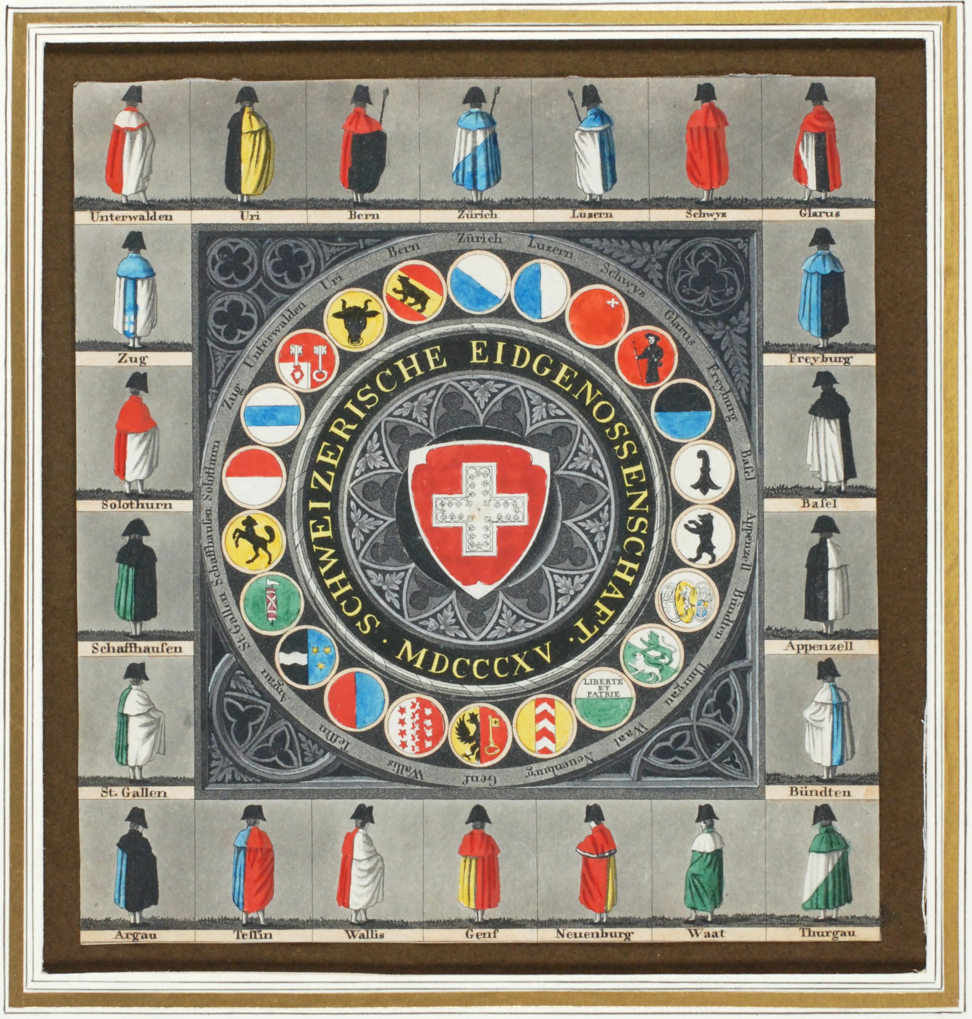
The task focuses on segmenting and measuring Swiss cantonal coats of arms (Wappen) from a historical image to demonstrate the extraction of visually similar objects. This is relevant for studying and preserving cultural symbols. The objective is to accurately detect, segment, and measure these objects using image processing techniques. The image comes from the article Liste der Wappen und Fahnen der Schweizer Kantone.
14: Segment the objects
Segment the objects using suitable 1-2 methods. Output the results as labeled images (binary or 1 label per class).
image_path = 'img/wappen.jpg'
image = cv2.imread(image_path)
gray_image = cv2.cvtColor(image, cv2.COLOR_BGR2GRAY)
# Apply Thresholding Methods
# Standard Binary Thresholding
_, binary_thresh = cv2.threshold(gray_image, 125, 255, cv2.THRESH_BINARY)
# Otsu's Thresholding
_, otsu_thresh = cv2.threshold(gray_image, 0, 255, cv2.THRESH_BINARY + cv2.THRESH_OTSU)
# Adaptive Thresholding
adaptive_thresh = cv2.adaptiveThreshold(
gray_image, 255, cv2.ADAPTIVE_THRESH_MEAN_C, cv2.THRESH_BINARY, 11, 2
)
# Store thresholding results with associated HoughCircles parameters
threshold_methods = [
("Standard Binary Threshold", binary_thresh, {"dp": 1.1, "minDist": 70, "param1": 30, "param2": 35, "minRadius": 50, "maxRadius": 80}),
("Otsu's Threshold", otsu_thresh, {"dp": 0.9, "minDist": 70, "param1": 50, "param2": 30, "minRadius": 40, "maxRadius": 80}),
("Adaptive Threshold", adaptive_thresh, {"dp": 1, "minDist": 80, "param1": 50, "param2": 50, "minRadius": 50, "maxRadius": 80}),
("Gray Image", gray_image, {"dp": 1, "minDist": 80, "param1": 50, "param2": 60, "minRadius": 50, "maxRadius": 80}),
]
# Prepare outputs for visualization
output_images = []
binary_classifications = []
# Process each thresholded image with respective HoughCircles parameters
for name, thresh, hough_params in threshold_methods:
# Circle detection using provided parameters
circles = cv2.HoughCircles(
thresh,
cv2.HOUGH_GRADIENT,
dp=hough_params["dp"],
minDist=hough_params["minDist"],
param1=hough_params["param1"],
param2=hough_params["param2"],
minRadius=hough_params["minRadius"],
maxRadius=hough_params["maxRadius"],
)
# Draw circles on the original image
circled_image = image.copy()
binary_classification = np.zeros_like(thresh)
if circles is not None:
circles = np.uint16(np.around(circles))
for circle in circles[0, :]:
x, y, r = circle
cv2.circle(circled_image, (x, y), r, (0, 255, 0), 4)
#cirle mask with applied transparency
cv2.circle(binary_classification, (x, y), r, 255, -1) # Binary classification mask
# Store results
output_images.append((name, circled_image))
binary_classifications.append((name, binary_classification))
# Visualize the results
fig, axes = plt.subplots(3, len(threshold_methods), figsize=(18, 15))
for i, (name, thresh, _) in enumerate(threshold_methods):
# Row 1: Thresholded images
axes[0, i].imshow(thresh, cmap='gray')
axes[0, i].set_title(name)
axes[0, i].axis('off')
# Row 2: Original image with detected circles
axes[1, i].imshow(cv2.cvtColor(output_images[i][1], cv2.COLOR_BGR2RGB))
axes[1, i].set_title(f"Circles: {name}")
axes[1, i].axis('off')
# Row 3: Binary classification mask
axes[2, i].imshow(binary_classifications[i][1], cmap='gray')
axes[2, i].set_title(f"Binary Classification: {name}")
axes[2, i].axis('off')
plt.tight_layout()
plt.show()

The results demonstrate that using the raw gray image for circle detection provided the most accurate outcome, as it detected all the Wappen correctly without producing any false positives. Otsu's Threshold performed well, accurately capturing most Wappen, though it included some false positives. Both Binary Thresholds performed similar with the most false positives and negatives.
path = './img/wappen.jpg'
image = cv2.imread(path)
gray_image = cv2.cvtColor(image, cv2.COLOR_BGR2GRAY)
# Refine Hough Circle Transform parameters
refined_circles = cv2.HoughCircles(
gray_image,
cv2.HOUGH_GRADIENT,
dp=1.0,
minDist=80,
param1=50,
param2=60,
minRadius=50,
maxRadius=80
)
# Draw detected circles and extract regions
refined_circle_extractions = []
visualized_image = image.copy()
if refined_circles is not None:
refined_circles = np.uint16(np.around(refined_circles))
for circle in refined_circles[0, :]:
x, y, r = circle
# Draw the circle for visualization
cv2.circle(visualized_image, (x, y), r, (0, 255, 0), 4)
# Crop the region of the circle
crop = image[y - (r+3):y + (r+3), x - (r+3):x + (r+3)]
if crop.size > 0:
refined_circle_extractions.append(crop)
# Plot the refined image with circles
plt.figure(figsize=(10, 10))
plt.imshow(cv2.cvtColor(visualized_image, cv2.COLOR_BGR2RGB))
plt.title("Detected Circles")
plt.axis('off')
plt.show()
# Plot the extracted Wappen from refined circles
if refined_circle_extractions:
fig, axes = plt.subplots(1, len(refined_circle_extractions), figsize=(15, 5))
for i, extraction in enumerate(refined_circle_extractions):
axes[i].imshow(cv2.cvtColor(extraction, cv2.COLOR_BGR2RGB))
axes[i].axis('off')
plt.tight_layout()
plt.show()
else:
print("No refined circles were detected. Further adjustment may be needed.")


Precision and Recall
These metrics evaluate the ability to correctly detect Wappen:
- Precision: Proportion of correctly detected Wappen out of all detected Wappen.
- Recall: Proportion of correctly detected Wappen out of all actual Wappen.
The formulas are:
$$ \text{Precision} = \frac{\text{True Positives}}{\text{True Positives} + \text{False Positives}} $$$$ \text{Recall} = \frac{\text{True Positives}}{\text{True Positives} + \text{False Negatives}} $$kpis = [
{'true positive': 13, 'false positive': 4, 'true negative': 0, 'false negative': 9, 'name': 'Standard Binary Threshold'},
{'true positive': 15, 'false positive': 4, 'true negative': 0, 'false negative': 7, 'name': "Otsu's Threshold"},
{'true positive': 16, 'false positive': 2, 'true negative': 0, 'false negative': 6, 'name': 'Adaptive Threshold'},
{'true positive': 22, 'false positive': 0, 'true negative': 0, 'false negative': 0, 'name': 'Gray Image'},
]
# Calculate and print Precision, Recall
for kpi in kpis:
print(f"{kpi['name']}: Precision = {kpi['true positive'] / (kpi['true positive'] + kpi['false positive']):.2f}, Recall = {kpi['true positive'] / (kpi['true positive'] + kpi['false negative']):.2f}")
Standard Binary Threshold: Precision = 0.76, Recall = 0.59
Otsu's Threshold: Precision = 0.79, Recall = 0.68
Adaptive Threshold: Precision = 0.89, Recall = 0.73
Gray Image: Precision = 1.00, Recall = 1.00
15: Morphological Operations
Improve the label masks using morphological operations. Show the intermediate results of your applied operations in individual images. Show that you have only changed the objects minimally (e.g. no shifts, reductions or enlargements) Can the periodicity of your pattern be made visible via an auto-correlogram? Visualize the results appropriately. Observe, interpret and discuss in 2-3 sentences.
cimage = cv2.cvtColor(image[450:700, 600:1200], cv2.COLOR_BGR2GRAY)
plt.imshow(cv2.cvtColor(cimage, cv2.COLOR_BGR2RGB))
gray_image = cimage
_, binary_thresh = cv2.threshold(gray_image, 180, 255, cv2.THRESH_BINARY)
contours, _ = cv2.findContours(binary_thresh, cv2.RETR_EXTERNAL, cv2.CHAIN_APPROX_SIMPLE)
labeled_mask = np.zeros_like(gray_image, dtype=np.uint8)
individual_masks = []
for i, contour in enumerate(contours, start=1):
individual_mask = np.zeros_like(gray_image, dtype=np.uint8)
cv2.drawContours(individual_mask, [contour], -1, 255, -1)
cv2.drawContours(labeled_mask, [contour], -1, i, -1)
individual_masks.append(individual_mask)
plt.figure(figsize=(10, 5))
plt.imshow(labeled_mask, cmap='grey')
plt.title("Labeled Mask")
plt.axis('off')
plt.show()


def apply_morphological_operations_with_differences(mask, kernel_size=(3, 3), iterations=1, min_size=10000):
# Structuring element (kernel)
kernel = np.ones(kernel_size, np.uint8)
# Perform morphological operations
operations = {
"Original Mask": mask,
"Erosion": cv2.erode(mask, kernel, iterations=iterations),
"Dilation": cv2.dilate(mask, kernel, iterations=iterations),
"Opening (Erosion + Dilation)": cv2.morphologyEx(mask, cv2.MORPH_OPEN, kernel),
"Closing (Dilation + Erosion)": cv2.morphologyEx(mask, cv2.MORPH_CLOSE, kernel),
}
# Filter small objects
filtered_mask = np.zeros_like(mask)
contours, _ = cv2.findContours(operations["Closing (Dilation + Erosion)"], cv2.RETR_EXTERNAL, cv2.CHAIN_APPROX_SIMPLE)
for contour in contours:
if cv2.contourArea(contour) >= min_size:
cv2.drawContours(filtered_mask, [contour], -1, 255, -1)
operations["Filtered Mask (Min Size)"] = filtered_mask
# Prepare a plot with refined mask and differences side-by-side
fig, axes = plt.subplots(len(operations), 2, figsize=(15, 4 * len(operations)))
for i, (name, result) in enumerate(operations.items()):
# Display refined mask
axes[i, 0].imshow(result, cmap='gray')
axes[i, 0].set_title(name)
axes[i, 0].axis('off')
# Display difference image
if name != "Original Mask":
diff = cv2.absdiff(mask, result)
axes[i, 1].imshow(diff, cmap='hot')
axes[i, 1].set_title(f"Difference: {name}")
axes[i, 1].axis('off')
else:
axes[i, 1].axis('off') # Skip difference for original mask
plt.tight_layout()
plt.show()
return operations
operations_result = apply_morphological_operations_with_differences(labeled_mask)

The results show that morphological operations like erosion, dilation, opening, and closing effectively refined the labeled mask, removing small noise and improving object boundaries while making minimal changes. I did not use the mask from yesterday as it was generated using perfect circles from Hough Circle detection, which would not benefit meaningfully from morphological refinements.
16: Morphological Operations Explained
For each operation used, explain in 1-2 sentences why you are using this operation. Observe, interpret and discuss in 2-3 sentences.
Erosion:
- Why: Erosion removes small noise and shrinks the boundaries of objects, which helps eliminate irrelevant small details that might have been falsely detected during segmentation.
- Parameters: A 3x3 kernel was chosen because it is small enough to avoid over-shrinking the Wappen, and 1 iteration was used to minimize the impact on object size.
Dilation:
- Why: Dilation expands the boundaries of objects, which helps recover details lost during erosion and fills small gaps within the objects.
- Parameters: A 3x3 kernel with 1 iteration was chosen to slightly expand the Wappen without merging separate objects.
Opening (Erosion + Dilation):
- Why: Opening removes small, isolated noise while preserving the shape of the Wappen. This operation ensures cleaner masks without impacting meaningful details.
- Parameters: A 3x3 kernel was used as it effectively removes noise while maintaining object integrity.
Closing (Dilation + Erosion):
- Why: Closing fills small gaps or holes within the Wappen, which improves the continuity of the object boundaries and ensures the masks are fully closed.
- Parameters: A 3x3 kernel was used to smooth boundaries and close minor imperfections without introducing distortions.
Filtered Mask (Min Size):
- Why: This operation removes any detected regions smaller than a specified minimum size, ensuring that only relevant Wappen are retained in the mask.
- Parameters: A minimum size of 10000 pixels was chosen to remove irrelevant noise while keeping all actual Wappen intact.
17: Measure The Objects
Think about which 2-3 properties you can use to measure the objects in the most characteristic way. Extract the individual objects, count and measure the 2-3 properties of your extracted objects using suitable methods.
kernel = np.ones((3,3), np.uint8)
mask = cv2.morphologyEx(labeled_mask, cv2.MORPH_OPEN, kernel, iterations=2)
original_image = cimage
# Find contours of objects
contours, _ = cv2.findContours(mask, cv2.RETR_EXTERNAL, cv2.CHAIN_APPROX_SIMPLE)
measurements = []
object_images = []
for i, contour in enumerate(contours):
# Calculate properties
area = cv2.contourArea(contour)
perimeter = cv2.arcLength(contour, True)
circularity = (4 * np.pi * area) / (perimeter ** 2) if perimeter > 0 else 0
# Get bounding box for object
x, y, w, h = cv2.boundingRect(contour)
cropped_object = original_image[y:y+h, x:x+w]
# Save properties and object image
measurements.append({"Wappen": i+1, "Area": area, "Perimeter": perimeter, "Circularity": circularity})
object_images.append(cropped_object)
# Convert measurements to DataFrame
results_df = pd.DataFrame(measurements)
filtered_results = results_df.where(results_df['Area'] > 9000).dropna()
print(filtered_results)
# Filter extracted objects
filtered_objects = [object_images[int(i)-1] for i in filtered_results["Wappen"]]
# Create a new filtered labeled mask
filtered_labeled_mask = np.zeros_like(labeled_mask)
for idx in filtered_results["Wappen"]:
contour = contours[int(idx)-1]
cv2.drawContours(filtered_labeled_mask, [contour], -1, int(idx), -1)
# Display the filtered labeled mask
plt.figure(figsize=(10, 5))
plt.imshow(filtered_labeled_mask, cmap='gray')
plt.title("Closing (Dilation + Erosion) and (Area > 9000)")
plt.axis('off')
plt.show()
# Plot the filtered extracted objects
fig, axes = plt.subplots(1, len(filtered_objects), figsize=(15, 5))
for i, obj in enumerate(filtered_objects):
axes[i].imshow(cv2.cvtColor(obj, cv2.COLOR_BGR2RGB))
axes[i].set_title(f"Wappen {i+1}")
axes[i].axis('off')
plt.tight_layout()
plt.show()
stats_summary = filtered_results.describe()
print(stats_summary)
Wappen Area Perimeter Circularity 18 19.0 12237.5 414.232536 0.896219 19 20.0 12271.0 415.646749 0.892567 20 21.0 24498.0 1115.744291 0.247293


Wappen Area Perimeter Circularity count 3.0 3.000000 3.000000 3.000000 mean 20.0 16335.500000 648.541192 0.678693 std 1.0 7068.952203 404.610370 0.373608 min 19.0 12237.500000 414.232536 0.247293 25% 19.5 12254.250000 414.939642 0.569930 50% 20.0 12271.000000 415.646749 0.892567 75% 20.5 18384.500000 765.695520 0.894393 max 21.0 24498.000000 1115.744291 0.896219
The best mask generated yesterday detected overlaping circles as single objects. Which is obvious when looking at the mesurements. The results suggest the need to incorporate the watershed algorithm to further separate overlapping circles for improved segmentation accuracy.
# Refine the mask using the watershed algorithm
dist_transform = cv2.distanceTransform(labeled_mask, cv2.DIST_L2, 5)
_, markers = cv2.threshold(dist_transform, 0.09 * dist_transform.max(), 255, 0)
markers = np.uint8(markers)
_, markers = cv2.connectedComponents(markers)
markers = markers + 1
segmented_mask = cv2.watershed(cv2.cvtColor(original_image, cv2.COLOR_GRAY2BGR), markers)
# Create final separated mask
final_separated_mask = np.zeros_like(mask)
for label in range(2, np.max(segmented_mask) + 1): # Skip background and undefined regions
final_separated_mask[segmented_mask == label] = 255
# Refine the separated mask further using morphological operations
kernel = np.ones((3, 3), np.uint8)
refined_mask = cv2.morphologyEx(final_separated_mask, cv2.MORPH_OPEN, kernel, iterations=2)
# Find contours of objects in the refined mask
contours, _ = cv2.findContours(refined_mask, cv2.RETR_EXTERNAL, cv2.CHAIN_APPROX_SIMPLE)
# Initialize results and object images
measurements = []
object_images = []
for i, contour in enumerate(contours):
# Calculate properties
area = cv2.contourArea(contour)
perimeter = cv2.arcLength(contour, True)
circularity = (4 * np.pi * area) / (perimeter ** 2) if perimeter > 0 else 0
# Get bounding box for object
x, y, w, h = cv2.boundingRect(contour)
cropped_object = original_image[y:y+h, x:x+w]
# Save properties and object image
measurements.append({"Wappen": i+1, "Area": area, "Perimeter": perimeter, "Circularity": circularity})
object_images.append(cropped_object)
# Convert measurements to DataFrame
results_df = pd.DataFrame(measurements)
# Filter results for significant areas
filtered_results = results_df.where(results_df['Area'] > 9000).dropna()
print(filtered_results)
# Filter extracted objects
filtered_objects = [object_images[int(i)-1] for i in filtered_results["Wappen"]]
# Create a new filtered labeled mask with minimal labels
filtered_labeled_mask = np.zeros_like(refined_mask)
for idx in range(1, len(filtered_objects) + 1):
contour = contours[idx - 1]
cv2.drawContours(filtered_labeled_mask, [contour], -1, idx, -1)
# Display the filtered labeled mask in black and white
plt.figure(figsize=(10, 5))
plt.imshow(filtered_labeled_mask, cmap='gray')
plt.title("Watershed and Closing (Dilation + Erosion) and (Area > 9000)")
plt.axis('off')
plt.show()
# Plot the filtered extracted objects
fig, axes = plt.subplots(1, len(filtered_objects), figsize=(15, 5))
for i, obj in enumerate(filtered_objects):
axes[i].imshow(cv2.cvtColor(obj, cv2.COLOR_BGR2RGB))
axes[i].set_title(f"Wappen {i+1}")
axes[i].axis('off')
plt.tight_layout()
plt.show()
# Display the filtered statistical summary
stats_summary = filtered_results.describe()
print(stats_summary)
Wappen Area Perimeter Circularity 0 1 10263.5 380.090400 0.892753 1 2 10283.0 380.676188 0.891699 2 3 9389.0 364.676187 0.887185 3 4 10294.5 380.918828 0.891559


Wappen Area Perimeter Circularity count 4.000000 4.000000 4.000000 4.000000 mean 2.500000 10057.500000 376.590401 0.890799 std 1.290994 445.850311 7.950418 0.002468 min 1.000000 9389.000000 364.676187 0.887185 25% 1.750000 10044.875000 376.236847 0.890466 50% 2.500000 10273.250000 380.383294 0.891629 75% 3.250000 10285.875000 380.736848 0.891963 max 4.000000 10294.500000 380.918828 0.892753
Using the watershed algorithm combined with other morphological operations, I successfully separated overlapping circles into distinct objects. The filtered labeled mask now accurately represents individual circles without overlap, and the statistical measurements show the segmentation's precision (mean circularity = 0.891). Notice the circularity in the first measurements were better, mean 0.894 for the not overlaping circles.
Circularity is a measured as:
$$ \text{Circularity} = \frac{4 \pi \cdot \text{Area}}{\text{Perimeter}^2} $$Values close to 1 indicate a shape is very circular, while lower values signify irregular or elongated shapes.
18: Representative Skeleton
Create a minimal but representative skeleton of one of your objects and output the number of pixels of the skeleton.
from skimage.morphology import skeletonize
wapden_n = 3
binary_mask = (filtered_labeled_mask == wapden_n)
skeleton = skeletonize(binary_mask)
skeleton_pixels = np.sum(skeleton)
# Display the skeleton
plt.figure(figsize=(10, 5))
plt.imshow(skeleton, cmap='gray')
plt.title(f"Skeleton of Wappen {wapden_n} (Pixels: {skeleton_pixels})")
plt.axis('off')
plt.show()
# Output the number of skeleton pixels
print(f"Number of pixels in the skeleton of Wappen {wapden_n} is {skeleton_pixels}")

Number of pixels in the skeleton of Wapen 3 is 1
Skeletonization reduces an object to its minimal form while maintaining its shape and connectivity.
Here, the number of skeleton pixels is used as a metric to evaluate the minimal representation of the object.
The skeleton extracted successfully preserves the circular structure of the object while minimizing the pixel count to 1 pixel.
The skeleton is both minimal and representative, which can be shown by reconstructing the shape of the wappen from the skeleton.
from skimage.morphology import skeletonize, dilation, disk
from skimage.metrics import structural_similarity as ssim
def iterative_best_fit(skeleton, original_mask, max_iterations=56, iou_threshold=0.999):
"""
Iteratively dilates the skeleton to fit the original mask and stops when the IoU score stabilizes.
Parameters:
skeleton (ndarray): The skeletonized object (binary mask).
original_mask (ndarray): The original object mask (binary mask).
max_iterations (int): Maximum number of iterations for dilation.
iou_threshold (float): IoU threshold to stop early.
Returns:
best_fit (ndarray): Dilated mask that best fits the original.
best_iou (float): IoU score of the best fit.
iterations (int): Number of iterations taken to reach the best fit.
"""
current_mask = skeleton.copy()
best_iou = 0
best_fit = current_mask
iterations = 0
for i in range(1, max_iterations + 1):
# Perform dilation
current_mask = skeleton.copy()
current_mask = dilation(current_mask, disk(i))
# Calculate IoU
intersection = np.logical_and(original_mask, current_mask)
union = np.logical_or(original_mask, current_mask)
iou = np.sum(intersection) / np.sum(union)
# Update best IoU and mask if improved
if iou > best_iou:
best_iou = iou
best_fit = current_mask.copy()
iterations = i
# Stop if IoU reaches threshold
if iou >= iou_threshold:
break
return best_fit, best_iou, iterations
# Skeletonize the selected object
binary_mask = (filtered_labeled_mask == wapden_n)
skeleton = skeletonize(binary_mask)
# Run iterative best fit
best_fit, best_iou, num_iterations = iterative_best_fit(skeleton, binary_mask)
# Create color overlay
overlap = np.zeros((binary_mask.shape[0], binary_mask.shape[1], 3), dtype=np.uint8)
# Define colors
both_color = [0, 255, 0] # Green: Both masks match
original_only = [255, 0, 0] # Red: Present only in original
reconstructed_only = [0, 0, 255] # Blue: Present only in reconstructed
# Build the overlap mask
overlap[np.logical_and(binary_mask, best_fit)] = both_color # True Positives
overlap[np.logical_and(binary_mask, ~best_fit)] = original_only # False Negatives
overlap[np.logical_and(~binary_mask, best_fit)] = reconstructed_only # False Positives
# Display the overlay
plt.figure(figsize=(10, 10))
plt.imshow(overlap[60:-60, 405:-70])
plt.title("Overlap: Original vs Reconstructed (Green: Both, Red: Original Only, Blue: Reconstructed Only)")
plt.axis('off')
plt.show()
# Print results
print(f"(IoU) Intersection over Unon Score: {best_iou:.4f}")
# Compute Structural Similarity Index (SSIM) for perceptual comparison
ssim_score = ssim(binary_mask, best_fit, data_range=1)
# Display results
print(f"Structural Similarity Index (SSIM): {ssim_score:.4f}")

(IoU) Intersection over Unon Score: 0.9692
Structural Similarity Index (SSIM): 0.9906
The reconstructed object closely matches the original with a IoU Score of 0.9692, indicating strong overlap and minimal deviation. The Structural Similarity Index (SSIM) of 0.9906 further confirms that the reconstructed shape preserves the perceptual characteristics of the original object.
19: Discussion
Discuss your choice of methods and parameters, as well as your findings and results in approx. 150 words. Are the results useful for the application?
The chosen methods effectively segmented and analyzed the Wappen (coat of arms). The watershed algorithm was used to separate overlapping objects, combined with morphological operations like opening and closing to remove noise while preserving object boundaries. These methods were selected for their reliability in object separation and refinement.
Key parameters, such as the distance transform threshold (0.09) and kernel size, were adjusted to achieve clean segmentation. The best parameters were found by trial and error. Skeletonization was applied to create minimal representations of the objects, capturing their essential structure. The IoU (0.9692) and SSIM (0.9906) metrics confirmed the accuracy of the reconstructed masks compared to the originals.
I think the results are suitable for the use case, as the skeletons and refined masks accurately represent the Wappen. The visual overlap and quantitative metrics validate the methods, ensuring reliable segmentation and analysis for further processing.